저번 포스트에 이어서 강화학습 본격적으로 공부하기 전 기초를 상기시키자.
1) Basic rules of partial differentiation
: 우리가 derivatives를 vectors \( x \in R^{n} \)에 대하여 계산할 때 항상 주의해야 한다.
-> 우리의 gradient는 vector와 matices를 포함한다.
-> 다음의 production, sum, chain 규칙을 따른다.

2) Chain rules
: a function \( f : R^{2} \rightarrow R \)이 두 변수 \( x_{1}, x_{2} \)에 대한 함수라고 하자.
-> 이 때 \( x(t) \) 자체도 \( t \)에 대한 함수이다.
-> 우리는 \( f \)의 gradient를 \( t \)에 대해 계산하고자 한다. 이때 chain rule이 적용된다.
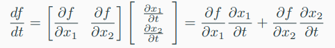
-> 여기서 \( d \)는 gradient를 \( \partial \)은 partial derivative를 나타낸다.
3) Multivariable vector-valued functions
: 우리는 vector-valued function \( f : R^{n} \rightarrow R^{m} \)에 대한 gradient 개념을 일반화할 것이다.
-> 이때 \( n > 1, m > 1 \)이고, \( x = [x_{1} x_{2} \cdots x_{n} ]^{T} \in R^{n}\)이다.
-> 따라서, 해당 조건을 만족하는 함수 \( f \)는 다음과 같이 주어진다.
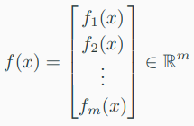
-> 여기에서 \( f_{i}(x) : R^{n} \rightarrow R \). // n차인 vector \( x \)를 1차인 element \( f_{i} \)로 보내주니까!
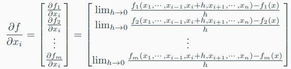
-> 해당 함수의 \( x_{i} \in R ( i = 1, 2, \cdots, n ) \) 대한 the partial derivative of a vector-valued function \( f : R^{n} \rightarrow R^{m} \)은 다음과 같은 vector로 주어진다.
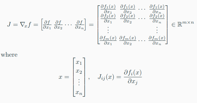
4) Jacobian for multivariable vector-valued functions
: 모든 first-order partial derivatives of a vector-valued function \( f : R^{n} \rightarrow R^{m} \)의 모음을 Jacobian이라고 한다.
-> The Jacobian J는 다음과 같다.
5) Gradient of a least-squared loss in a linear model
-> 다음과 같은 선형 모델을 가정하자.

-> 여기에서 \( \theta \in R^{n} \)은 parameter vector (to be determined)이고, \( \Phi \in R^{m \times n} \)은 input feasures, 그리고 \( y \in R^{m} \)은 corresponding observation이다.
-> 쉽게 말해서 계수, 입력, 출력을 나타낸다.
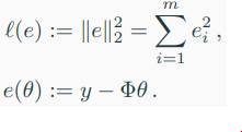
-> 이때 the loss and error fucntion을 다음과 같이 정의한다.
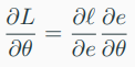
-> 우리는 \( \frac{\partial L}{\partial \theta} \)를 찾고자 한다.
=> 여기서 chain rule이 사용된다.
-> \( L(\theta) := (l \circ e)(\theta) \)는 least-squares loss function이다.
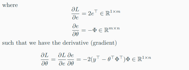
-> \( L \)의 \( \theta \)에 대한 gradient는 다음과 같다.
-> 각각에 대한 derivative는 다음과 같다.
6) Gradient of vectors with respect to matrices (or vectors)
: 이번엔 matrices (of vectors)에 대한 vectors의 gradient를 알아보자.
-> 다음과 같은 모델을 가정한다.
\(f = Ax\)
-> 여기에서 \( A \in R^{m \times n}\)이고, 우리가 찾는 graient는 다음과 같다.
\( \frac{df}{dA} \in R^{m \times (m \times n)}\)
-> 정의에 의해, gradient는 partial derivatives들의 모음이다.

7) Gradient of matrices with respect to matrices
: 이번엔 matrices에 대한 matrices의 gradient를 알아보자.
-> 다음과 같은 조건으 가정한다.
-> \( R \in R^{m \times n} \) and \( f : R^{m \times n} \rightarrow R^{n \times n} \) with
\( f(R) = R^{T}R =: K \in R^{n \times n} \)
-> where we seek the gradient
\( \frac{dK}{dR} \)
8) Hessian matrix
: derivatives of higher order에 대해 계산해야할 때, 예를 들어 Newton's Method for optimization을 사용할 때 second-order derivatives를 요구한다.
-> The Hessian은 모든 second-order partial derivatives의 모음이다.
-> 만약, \( f(x, y) \)가 twice (continuosly) differentiable 함수라면
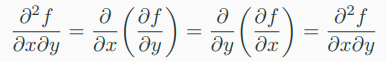
-> 이때 differentiation의 차수는 중요하지 않다.
-> 해당 식과 일치하는 Hessian matrix는 다음과 같다.
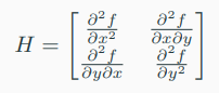
-> \( H \)는 symmetric하고, 일반적으로 \( x \in R^{n} \)이고 \( f : R^{n} -> R \)일 때, \( H \in R^{n \times n} \) symmetric matrix이다.
9) Multivariate Taylor Series
: 이변수 함수의 Taylor 급수는 어떻게 구할까?
-> 일변수 함수의 Taylor 급수는 다음과 같았다.

-> 이변수 함수의 Taylor 급수는 마찬가지의 방법으로 전개한다.
-> \( (x-a) \), \( (x-b) \)의 Taylor 급수를 전개하려고 할 때

-> 각각 미분해주고,

-> 위와 같이 다음 항들은 4가지 경우에 대한 미분을 해주어야한다.
%% 다시 한번 정리
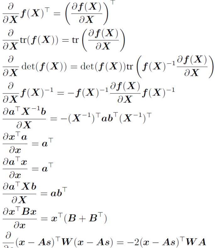
10) Useful identities for computing gradients
'Study > Reinforcement learning' 카테고리의 다른 글
| 강화학습_(6) - Neural Network의 학습 방법 - Gradient descent, Back-propagation (0) | 2019.10.30 |
|---|---|
| 강화학습_(5) - 머신 러닝 분류 - 지도 학습, 비지도 학습, 강화 학습 (0) | 2019.10.30 |
| 강화학습_(4) - Math Preliminary_1 (0) | 2019.10.22 |
| 강화학습_(3) - 시그모이드 (Sigmoid)함수 정의 (0) | 2019.10.21 |
| 강화학습_(2) - Python 기초_4 (0) | 2019.10.20 |